Module - 5 Dynamic-Routing
2026-09-19 21:19
Tags: #Network
Author: Duke Hsu
Topic
- Dynamic Routing Protocol
- Distance Vector Dynamic Routing
- Link-State Dynamic Routing
1. Dynamic Routing Protocol
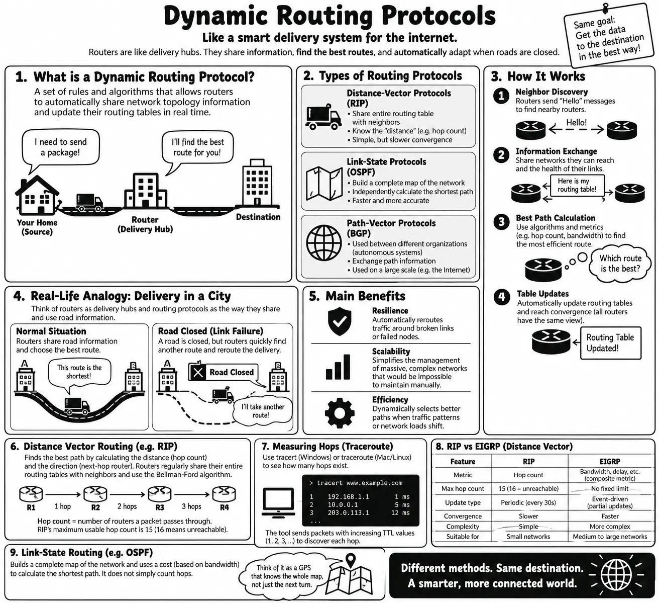
A Dynamic Routing Protocol is a set of rules and algorithms that allows routers to automatically share network topology information and update their routing tables in real time .
1.1 Types of Routing Protocol
1.1.1 Distance-Vector Protocols
Routing Information Protocol (RIP)
Routers share their entire routing table or summaries with their direct neighbors. They know the "Distance" (e.g. hop count) to a destination, but not the full network map.
1.1.2 Link-State Protocols
Open Shortest Path First(OSPF)
Every router builds a complete map of the entire network topology and independently calculates the shortest path to each destination .
1.1.3 Path-Vector Protocols
Border Gateway Protocol(BGP)
Used to exchange routing information between entirely separate, large-scale administrative domains or autonomous systems.
1.2 How It Works
- Neighbor Discovery: Routers send out special messages (like "Hello" packets) to discover neighboring routers on the network .
- Information Exchanges: They share details about the networks they can reach and the health of their connections.
- Best Path Calculation: Using built-in algorithms , each router calculates the most efficient route to every destination based on specific metrics like hop count or bandwidth
- Table Updates: Routers automatically update their routing tables to reflect the optimal paths and achieve convergence ( a state where all routers share a consistent view of the network )
1.3 Main Benefits
- Resilience: Automatically rerouters traffic around broken links or failed nodes.
- Scalability: Simplifies the management of massive, complex networks that would be impossible to maintain manually .
- Efficiency: Dynamically selects better paths when traffic patterns or network loads shift.
2. Distance Vector Routing
Distance Vector Routing is a dynamic routing protocol that finds the best path to a destination network by calculating both the distance(how far, such as hop count) and the direction(the next-hop router and exit interface).
2.1 How It Works
- Routing Tables: Every router keeps a table listing all know destinations, the cost to reach them , and the next hop to get there.
- Sharing with Neighbors: Routers regularly share their entire routing tables(or parts of them ) with their direct neighbors in a process often called "routing by rumor"
- Bellman-Ford Algorithm: Each router recalculates its best paths using the Bellman-Ford equation based on the updates received from neighbors.
- Convergence: The network reaches "convergence" when all routers share consistent, up-to-date views of the network topology .
2.2 Hop Count
In networking , calculating a router Hop count means counting how many Layer 3 network devices with IP addresses , mainly routers, a data packet passes through from the source to the destination .
Simply put, every time a packet is forwarded by a router , the hop count increases by 1. Switches and hubs operate at the Data Link Layer or Physical Layer, so they are not counted as hops.
How can we measure and calculate hops in practice?
To check how many hops exist between your computer and a destination server, the most commonly used commands are:
-
Windows:
tracert [destination IP or domain] -
Mac / Linux:
traceroute [destination IP or domain]
Basic principle:
-
The tracing tool first sends a packet with a TTL (Time to Live) value of 1.
-
When the packet reaches the first router, the TTL decreases to 0. The router then discards the packet and sends a timeout message back to your computer. This records Hop 1.
-
Next, the tool sends another packet with the TTL set to 2, allowing it to reach and record Hop 2.
-
This process continues until the packet successfully reaches the destination, allowing the tool to display the IP address and delay of each hop along the route.
How do routers calculate hops internally?
At the network level, routers use Routing Protocols to determine the best path and build their routing tables.
-
Distance Vector Protocols, such as RIP (Routing Information Protocol):
-
RIP uses Hop Count as its main metric for choosing the best path.
-
For example, if Path A has 3 hops and Path B has 5 hops, RIP will choose Path A.
-
The maximum usable hop count in RIP is normally 15. A hop count of 16 means the destination is unreachable.
-
-
Link-State Protocols, such as OSPF (Open Shortest Path First):
-
OSPF does not simply count hops.
-
Instead, it uses Cost as its routing metric, which is mainly calculated based on interface bandwidth, to determine the best path.
-
2.3 Key Characteristics
- Periodic Updates: Tables are sent out at regular time intervals (r.g. every 30 seconds)
- Metric: Uses hop count ( the number of routers passed through ) as the primary measure of distance.
- Common Examples: Protocols like Routing information Protocol (RIP) use this approach
2.3 Types of Distance Vector Routing Protocols
Difference Between RIP and EIGRP
| RIP | EIGRP |
|---|---|
| RIP stands for Routing Information Protocol. | EIGRP stands for Enhanced Interior Gateway Routing Protocol. |
| RIP works on Bellman Ford algorithm. | EIGRP works on DUAL(Diffusing Update Algorithm) Algorithm. |
| It is a industry standard dynamic routing protocol. | It is a Cisco standard routing protocol. |
| It is basically use for smaller size organization. | It is basically use for larger size organization as compared to RIP. |
| RIP is a distance vector protocol. | EIGRP is derived from Integrated Gateway Routing Protocol. |
| It allow maximum hop count upto 15. | It allow maximum hop count upto 255. |
| It’s administrative distance is 120. | It’s administrative distance is 90. |
| It is not a more intelligent dynamic routing protocol. | It is a more intelligent routing protocol than RIP. |
| It calculates the metric in terms of Hop Count. | It calculates the metric in terms of bandwidth and delay. |
| RIP routing protocol creates two table in the router: Routing Table, and Topology Table. | EIGRP routing protocol creates three table In the router: Neighbor Table, Topology Table, and Routing Table. |
| The symbol "R" is used to denote RIP in the routing table. | The symbol "D" is used to denote EIGRP in the routing table. |
| A separate administrative boundary is not possible to create in the RIP routing protocol. | A separate administrative boundary is possible to create in the EIGRP routing protocol using autonomous system (AS) No. |
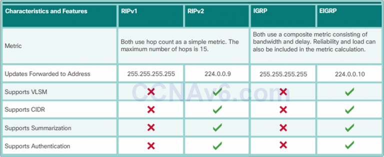
2.4 Advantages & Disadvantages
- Pros: Easy to step up , low resource use, and works well in smaller networks.
- Cons: Slower to adapt to network changes (slow convergence ) and prone to routing loops or "count-to-infinity" problems
3. Link-State Routing Protocol Operation
Link-state routing protocols allow every router to build a complete topological map of the network and independently calculate the best path to every destination .
Common examples include Open Shortest Path First (OSPF) and Intermediate System to Intermediate System(IS-IS)
3.1 Key Operational Steps
- Neighbor Discovery(Hello Protocol):
- Routers end periodic Hello packets to find directly connected neighbors and establish adjacencies. If Hello messages stop , the neighbor is assumed dead.
- Building Link-State Information:
- Each router gathers information about its local links, costs, and active neighbors, packaging this data into a Link-State Advertisement(LSA) or Link-State Packet(LSP)
- Reliable Flooding:
- Routers flood these LSAs to all adjacent neighbors, which in turn pass them along until every router in the area receives the exact same update.
- Database Synchronization:
- All routers store received LSAs in a local Link-State Database(LSDB)
- Shortest Path Calculation(Dijkstra's Algorithm):
- Using the LSDB as a complete network graph, each router independently runs Dijkstra's Shortest Path First (SPF) algorithm to calculate the optimal path to every destination.
- Routing Table Population:
- The results from the SPF tree are compiled to build the final IP routing table used for packet forwarding.
3.2 Advantages and Disadvantages
Advantages
- Builds a complete topological map of the network to determine the shortest path
- Floods the LSP immediately to achieve faster converge
- Only sends out LSP with new information when there is a change in the topology
- Uses the concept of areas and allows for summarization
Disadvantages
- Requires additional memory to maintain the database and SPF tree
- Requires more CPU processing to calculate the SPF algorithm and create a compete map of the topology
- Requires more bandwidth during initial startups of the routers and could be an issue on unstable networks
4. SPF Tree
An SPF Tree (Shortest Path First Tree) is a loop-free network map created by a router using the Shortest Path First (Dijkstra's) algorithm to find the best data paths.
How an SPF Tree Works in Networking
-
Root Node: The calculating router sits at the exact center (the root) of the network tree.
-
Branches and Leaves: All other routers, switches, and networks branch out like tree limbs based on distance and cost.
-
Cost Metric: Links are assigned a "cost" based on speed; faster connections have a lower cost and are chosen as the best path.
-
Routing Table: The router uses this finished tree to populate its routing table and forward network traffic efficiently.
Where It Is Used
-
OSPF (Open Shortest Path First): A common link-state routing protocol used in large IP networks.
-
IS-IS (Intermediate System-to-Intermediate System): Another major routing protocol that uses the same core algorithm to build shortest-path trees. [1]
References
https://www.logicmonitor.com/deep-dive/dynamic-routing-protocols/introduction
https://www.zenarmor.com/docs/network-basics/what-is-dynamic-routing
https://www.geeksforgeeks.org/computer-networks/difference-between-rip-and-eigrp/
https://itexamanswers.net/ccna-3-v6-0-study-material-chapter-5-dynamic-routing.html